Not really complete...

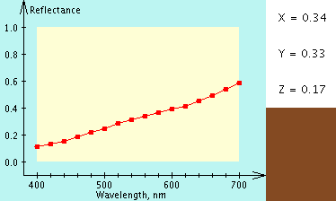
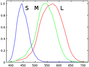
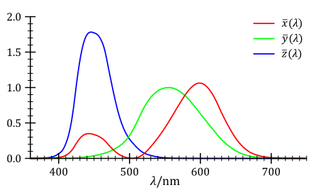
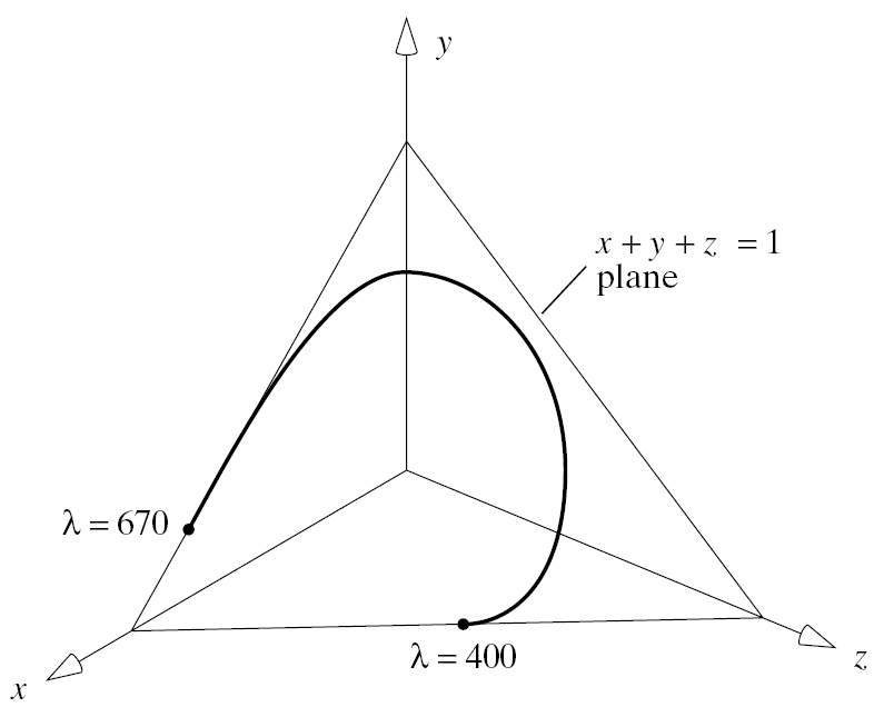
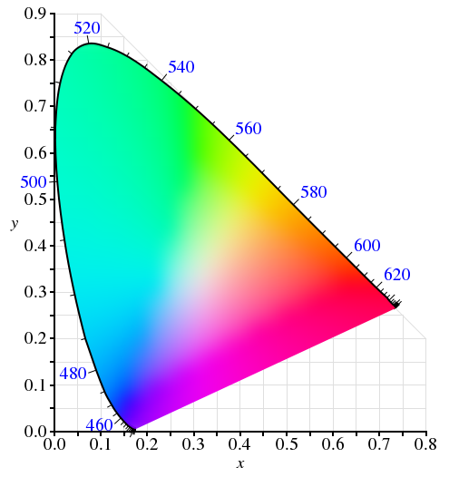
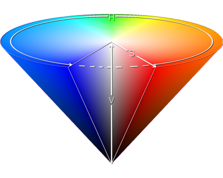
Colour notes here, transformations notes here.

Parametric Curves and Surfaces

Parametric Representation

eg. $latex C(t) = (x(t), y(t))$

Continuity

Parametric Continuity

• If the first derivative of a curve is continuous, we say it has C¹ continuity.

Geometric Continuity

• If the magnitude of the first derivative of a curve changes but the direction doesn't then, we say it has G¹ continuity.
• Curves need G2 continuity in order for a car to drive along them. (ie. not instantly change steering wheel angle at any points).

Control Points

Control points allow us to shape/define curves visually. A curve will either interpolate or approximate control points.

Natural Cubic Splines

• Interpolate control points.
• A cubic curve between each pair of control points
• Four unknowns,
  • • interpolating the two control points gives two,
    • requiring that derivatives match at end of points of these curves gives the other two.
• Moving one control point changes the whole curve (ie. no local control over the shape of the curve)

Bezier Curve

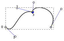
This Bezier curve shown has two segments, where each segment is defined by 4 control points. The curve interpolates two points and approximates the other two. The curve is defined by a Bernstein polynomial. In the diagram changing points 1 and 2 only affects that segment. Changing the corner points (0 and 3) each only affect the two segments that they boarder.

Some properties of Bezier Curves:

• Tangent Property. Tangent at point 0 is line 0 to 1, similarly for point 3.
• Convex Hull Property. The curve lies inside the convex hull of the control points. (The corollary of this is if the control points are colinear, the curve is a line.)
• They have affine invariance.
• Can't fluctuate more than their control polygon does.
• Bezier's are a special case of B-spline curves.

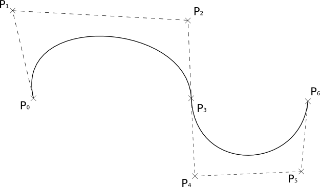
We can join two Bezier curves together to have C¹ continuity (where B₁(P₀, P₁, P₂, P₃) and B₂(P₀, P₁, P₂, P₃)) if P₃ - P₂ = P₄ - P₃. That is P₂, P₃,  and P₄ are colinear and P₃ is the midpoint of P₂ and P₄. To get G¹ continuity we just need P₂, P₃, and P₄ to be colinear. If we have G¹ continuity but not C¹ continuity the curve still won't have any corners but you will notice a "corner" if your using the curve for something else such as some cases in animation. [Also if the curve defined a road without G¹ continuity there would be points where you must change the steering wheel from one rotation to another instantly in order to stay on the path.]

De Casteljau Algorithm

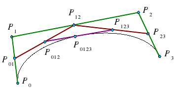
De Casteljau Algorithm is a recursive method to evaluate points on a Bezier curve.

To calculate the point halfway on the curve, that is t = 0.5 using De Casteljau's algorithm we (as shown above) find the midpoints on each of the lines shown in green, then join the midpoints of the lines shown in red, then the midpoint of the resulting line is a point on the curve. To find the points for different values of t, just use that ratio to split the lines instead of using the midpoints. Also note that we have actually split the Bezier curve into two. The first defined by P₀, P₀₁, P₀₁₂, P₀₁₂₃ and the second by P₀₁₂₃, P₁₂₃, P₂₃, P₃.

Curvature

The curvature of a circle is $latex \frac{1}{r}$.

The curvature of a curve at any point is the curvature of the osculating circle at that point. The osculating circle for a point on a curve is the circle that "just touches" the curve at that point. The curvature of a curve corresponds to the position of the steering wheel of a car going around that curve.

Uniform B Splines

Join with C2 continuity.

Any of the B splines don't interpolate any points, just approximate the control points.

Non-Uniform B Splines

Only invariant under affine transformations, not projective transformations.

Rational B Splines

Rational means that they are invariant under projective and affine transformations.

NURBS

Non-Uniform Rational B Splines

Can be used to model any of the conic sections (circle, ellipse, hyperbola)

=====================

3D

When rotating about an axis in OpenGL you can use the right hand rule to determine the + direction (thumb points in axis, finger indicate + rotation direction).

We can think of transformations as changing the coordinate system, where (u, v, n) is the new basis and O is the origin.

$latex \begin{pmatrix}u_x & v_x & n_x & O_x\ u_y & v_y & n_y & O_y\ u_z & v_z & n_z & O_z\ 0 & 0 & 0 & 1 \end{pmatrix}$

This kind of transformation in is known as a local to world transform. This is useful for defining objects which are made up of many smaller objects. It also means to transform the object we just have to change the local to world transform instead of changing the coordinates of each individual vertex. A series of local to world transformations on objects builds up a scene graph, useful for drawing a scene with many distinct models.

Matrix Stacks

OpenGL has MODELVIEW, PROJECTION, VIEWPORT, and TEXTURE matrix modes.

• glLoadIdentity() - puts the Identity matrix on the top of the stack
• glPushMatrix() - copies the top of the matrix stack and puts it on top
• glPopMatrix()

For MODELVIEW operations include glTranslate, glScaled, glRotated... These are post multiplied to the top of the stack, so the last call is done first (ie. a glTranslate then glScaled will scale then translate.).

Any glVertex() called have the value transformed by matrix on the top of the MODELVIEW stack.

Usually the hardware only supports projection and viewport stacks of size 2, whereas the modelview stack should have at least a size of 32.

The View Volume

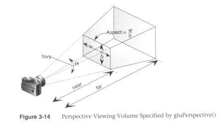
Can set the view volume using,(after setting the the current matrix stack to the PROJECTION stack

• glOrtho(left, right, bottom, top, near, far) 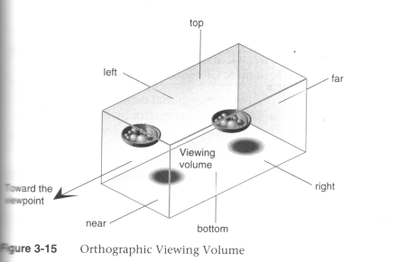(Source: Unknown)
• glFrustum(left, right, bottom, top, near, far) 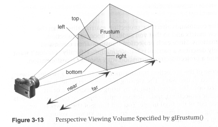(Source: Unknown)
• gluPerspective(fovy, aspect, zNear, zFar) (Source: Unknown)

In OpenGL the projection method just determines how to squish the 3D space into the canonical view volume.

Then you can set the direction using gluLookAt (after calling one of the above) where you set the eye location, a forward look at vector and an up vector.

When using perspective the view volume will be a frustum, but this is more complicated to clip against than a cube. So we convert the view volume into the canonical view volume which is just a transformation to make the view volume a cube at 0,0,0 of width 2. Yes this introduces distortion but this will be compensated by the final window to viewport transformation.

Remember we can set the viewport with glViewport(left, bottom, width, height) where x and y are a location in the screen (I think this means window, but also this stuff is probably older that modern window management so I'm not worrying about the details here.)

Visible Surface Determination (Hidden Surface Removal)

First clip to the view volume then do back face culling.

Could just sort the polygons and draw the ones further away first (painter's algorithm/depth sorting). But this fails for those three overlapping triangles.

Can fix by splitting the polygons.

BSP (Binary Space Partitioning)

For each polygon there is a region in front and a region behind the polygon. Keep subdividing the space for all the polygons.

Can then use this BSP tree to draw.

void drawBSP(BSPTree m, Point myPos{
   if (m.poly.inFront(myPos)) {
      drawBSP(m.behind, myPos);
      draw(m.poly);
      drawBSP(m.front, myPos);
   }else{
      drawBSP(m.front, myPos);
      draw(m.poly);
      drawBSP(m.behind, myPos);
   }
}

If one polygon's plane cuts another polygon, need to split the polygon.

You get different tree structures depending on the order you select the polygons. This does not matter, but some orders will give a more efficient result.

Building the BSP tree is slow, but it does not need to be recalculated when the viewer moves around. We would need to recalculate the tree if the polygons move or new ones are added.

BSP trees are not so common anymore, instead the Z buffer is used.

Z Buffer

Before we fill in a pixel into the framebuffer, we check the z buffer and only fill that pixel is the z value (can be a pseudo-depth) is less (large values for further away) than the one in the z buffer. If we fill then we must also update the z buffer value for that pixel.

Try to use the full range of values for each pixel element in the z buffer.

To use in OpenGL just do gl.glEnable(GL.GL_DEPTH_TEST) and to clear the z-buffer use gl.glClear(GL.GL_DEPTH_BUFFER_BIT).

Fractals

L-Systems

Line systems. eg. koch curve

Self-similarity

• Exact (eg. sierpinski trangle)
• Stochastic (eg. mandelbrot set)

IFS - Iterated Function System

================================================

Shading Models

There are two main types of rendering that we cover,

• polygon rendering
• ray tracing

Polygon rendering is used to apply illumination models to polygons, whereas ray tracing applies to arbitrary geometrical objects. Ray tracing is more accurate, whereas polygon rendering does a lot of fudging to get things to look real, but polygon rendering is much faster than ray tracing.

• With polygon rendering we must approximate NURBS into polygons, with ray tracing we don't need to, hence we can get perfectly smooth surfaces.
• Much of the light that illuminates a scene is indirect light (meaning it has not come directly from the light source). In polygon rendering we fudge this using ambient light. Global illumination models (such as ray tracing, radiosity) deal with this indirect light.
• When rendering we assume that objects have material properties which we denote k_(property).
• We are trying to determine I which is the colour to draw on the screen.

We start with a simple model and build up,

Lets assume each object has a defined colour. Hence our illumination model is $latex I = k_i$, very simple, looks unrealistic.

Now we add ambient light into the scene. Ambient Light is indirect light (ie. did not come straight from the light source) but rather it has reflected off other objects (from diffuse reflection). $latex I = I_a k_a$. We will just assume that all parts of our object have the same amount of ambient light illuminating them for this model.

Next we use the diffuse illumination model to add shading based on light sources. This works well for non-reflective surfaces (matte, not shiny) as we assume that light reflected off the object is equally reflected in every direction.

Lambert's Law

"intensity of light reflected from a surface is proportional to the cosine of the angle between L (vector to light source) and N(normal at the point)."

Gouraud Shading

Use normals at each vertex to calculate the colour of that vertex (if we don't have them, we can calculate them from the polygon normals for each face). Do for each vertex in the polygon and interpolate the colour to fill the polygon. The vertex normals address the common issue that our polygon surface is just an approximation of a curved surface.

To use gouraud shading in OpenGL use glShadeModel(GL_SMOOTH). But we also need to define the vertex normals with glNormal3f() (which will be set to any glVertex that you specify after calling glNormal).

Highlights don't look realistic as you are only sampling at every vertex.

Interpolated shading is the same, but we use the polygon normal as the normal for each vertex, rather than the vertex normal.

Phong Shading

Like gouraud, but you interpolate the normals and then apply the illumination equation for each pixel.

This gives much nicer highlights without needing to increase the number of polygons, as you are sampling at every pixel.

Phong Illumination Model

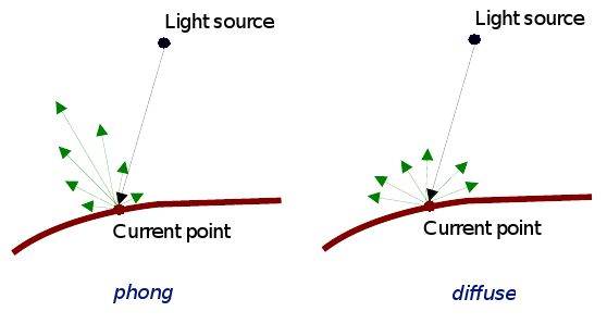
Diffuse reflection and specular reflection.

(Source: COMP3421, Lecture Slides.)

$latex I_s = I_l k_s \cos^n \left ( \alpha \right )$

n is the Phong exponent and determines how shiny the material (the larger n the smaller the highlight circle).

Flat shading. Can do smooth shading with some interpolation.

If you don't have vertex normals, you can interpolate it using the face normals of the surrounding faces.

Gouraud interpolates the colour, phong interpolates the normals.

Attenuation

inverse square is physically correct, but looks wrong because real lights are not single points as we usually use in describing a scene, and

For now I assume that all polygons are triangles. We can store the normal per polygon. This will reneder this polygon, but most of the time the polygon model is just an approximation of some smooth surface, so what we really want to do is use vertex normals and interpolate them for the polygon.

Ray Tracing

For each pixel on the screen shoot out a ray and bounce it around the scene. The same as shooting rays from the light sources, but only very few would make it into the camera so its not very efficient.

Each object in the scene must provide an intersection(Line2D) function and a normal (Point3D) function

Ray Tree

Nodes are intersections of a light ray with an object. Can branch intersections for reflected/refracted rays. The primary ray is the original ray and the others are secondary rays.

Shadows

Can do them using ray tracing, or can use shadow maps along with the Z buffer. The key to shadow maps is to render the scene from the light's perspective and save the depths in the Z buffer. Then can compare this Z value to the transformed Z value of a candidate pixel.

==============

Rasterisation

Line Drawing

DDA

• You iterate over x or y, and calculate the other coordinate using the line equation (and rounding it).
• If the gradient of the line is > 1 we must iterate over y otherwise iterate over x. Otherwise we would have gaps in the line.
• Also need to check if x1 is > or < x2 or equal and have different cases for these.

Bresenham

• Only uses integer calcs and no multiplications so its much faster than DDA.
• We define an algorithm for the 1st octant and deal with the other octant's with cases.
• We start with the first pixel being the lower left end point. From there there are only two possible pixels that we would need to fill. The one to the right or the one to the top right. Bresenham's algorithm gives a rule for which pixel to go to. We only need to do this incrementally so we can just keep working out which pixel to go to next.
• The idea is we accumulate an error and when that exceeds a certain amount we go up right, then clear the error, other wise we add to the error and go right.

We use Bresenham's algorithm for drawing lines this is just doing linear interpolation, so we can use Bresenham's algorithm for other tasks that need linear interpolation.

Polygon Filling

Scan line Algorithm

The Active Edge List (AEL) is initially empty and the Inactive Edge List (IEL) initially contains all the edges. As the scanline crosses an edge it is moved from the IEL to the AEL, then after the scanline no longer crosses that edge it is removed from the AEL.

To fill the scanline,

• On the left edge, round up to the nearest integer, with round(n) = n if n is an integer.
• On the right edge, round down to the nearest integer, but with round(n) = n-1 if n is an integer.

Its really easy to fill a triangle, so an alternative is to split the polygon into triangles and just fill the triangles.

===============

Anti-Aliasing

Ideally a pixel's colour should be the area of the polygon that falls inside that pixel (and is on top of other polygons on that pixel) times the average colour of the polygon in that pixel region then multiply with any other resulting pixel colours that you get from other polygons in that pixel that's not on top of any other polygon on that pixel.

Aliasing Problems

• Small objects that fall between the centre of two adjacent pixels are missed by aliasing. Anti-aliasing would fix this by shading the pixels a gray rather than full black if the polygon filled the whole pixel.
• Edges look rough ("the jaggies").
• Textures disintegrate in the distance
• Other non-graphics problems.

Anti-Aliasing

In order to really understand this anti-aliasing stuff I think you need some basic understanding of how a standard scene is drawn. When using a polygon rendering method (such as is done with most real time 3D), you have a framebuffer which is just an area of memory that stores the RGB values of each pixel. Initially this framebuffer is filled with the background colour, then polygons are drawn on top. If your rending engine uses some kind of hidden surface removal it will ensure that the things that should be on top are actually drawn on top.

Using the example shown (idea from http://cgi.cse.unsw.edu.au/~cs3421/wordpress/2009/09/24/week-10-tutorial/#more-60), and using the rule that if a sample falls exactly on the edge of two polygons, we take the pixel is only filled if it is a top edge of the polygon.

No Anti-Aliasing

With no anti-aliasing we just draw the pixel as the colour of the polygon that takes up the most area in the pixel.

Pre-Filtering

• We only know what colours came before this pixel, and we don't know if anything will be drawn on top.
• We take a weighted (based on the ratio of how much of the pixel the polygon covers) averages along the way. For example if the pixel was filled with half green, then another half red, the final anti-aliased colour of that pixel would determined by, Green (0, 1, 0) averaged with red (1, 0, 0) which is (0.5, 0.5, 0). If we had any more colours we would then average (0.5, 0.5, 0) with the next one, and so on.
• Remember weighted averages, $latex \frac{Aa + Bb}{A + B}$ where you are averaging $latex a$ and $latex b$ with weights $latex A$ and $latex B$ respectively.
• Pre-filtering is designed to work with polygon rendering because you need to know the ratio which by nature a tracer doesn't know (because it just takes samples), nor does it know which polygons fall in a given pixel (again because ray tracers just take samples).
• Pre-filtering works very well for anti-aliasing lines, and other vector graphics.

Post-Filtering

• Post-filtering uses supersampling.
• We take some samples (can jitter (stochastic sampling) them, but this only really helps when you have vertical or horizontal lines moving vertically or horizontally across a pixel, eg. with vector graphics)
• $latex \left ( \frac{6}{9} \right )$ of the samples are Green, and $latex \left ( \frac{3}{9} \right )$ are red. So we use this to take an average to get the final pixel colour of $latex \begin{pmatrix}\frac{1}{3}, & \frac{2}{3}, & 0\end{pmatrix}$
• We can weight these samples (usually centre sample has more weight). The method we use for deciding the weights is called the filter. (equal weights is called the box filter)
• Because we have to store all the colour values for the pixel we use more memory than with pre-filtering (but don't need to calculate the area ratio).
• Works for either polygon rendering or ray tracing.

Can use adaptive supersampling. If it looks like a region is just one colour, don't bother supersampling that region.

OpenGL

Often the graphics card will take over and do supersamling for you (full scene anti aliasing).

To get OpenGL to anti-alias lines you need to first tell it to calculate alpha for each pixel (ie. the ratio of non-filled to filled area of the pixel) using, glEnable(GL_LINE_SMOOTH) and then enable alpha blending to apply this when drawing using,

glEnable(GL_BLEND);
glBlendFunc(GL_SRC_ALPHA, GL_ONE_MINUS_SRC_ALPHA);

You can do post-filtering using the accumulation buffer (which is like the framebuffer but will apply averages of the pixels), and jittering the camera for a few times using accPerspective.

Anti-Aliasing Textures

A texel is a texture pixel whereas a pixel in this context refers to a pixel in the final rendered image.

When magnifying the image can use bilinear filtering (linear interpolation) to fill the gaps.

Mip Mapping

Storing scaled down images and choose closes and also interpolate between levels where needed. Called trilinear filtering.

Rip Mapping helps with non uniform scaling of textures. Anisotropic filtering is more general and deals with any non-linear transformation applied to the texture

Double Buffering

We can animate graphics by simply changing the framebuffer, however if we start changing the framebuffer and we cannot change it faster than the rate the screen will display the contents of the frame buffer, it gets drawn when we have only changed part of the framebuffer. To prevent this, we render the image to an off screen buffer and when we finish we tell the hardware to switch buffers.

Can do on-demand rendering (only refill framebuffer when need to) or continuois rendeing (draw method is called at a fixed rate and the image is redrawn regardless of whether the image needs to be updated.)

LOD

Mip Mapping for models. Can have some low poly models that we use when far away, and use the high res ones when close up.

Animation

Key-frames and tween between them to fill up the frames.

===============

Shaders

OpenGL 2.0  using GLSL will let us implement out own programs for parts of the graphics pipeline particularly the vertex transformation stage and fragment texturing and colouring stage.

Fragments are like pixels except they may not appear on the screen if they are discarded by the Z-buffer.

Vertex Shaders

• position tranformation and projection (set gl_Position), and
• lighting calculation (set gl_FrontColor)

Fragment Shaders

• interpolate vertex colours for each fragment
• apply textures
• etc.

set gl_FragColor.

Homogeneous Coordinates

Interestingly we can use the extra dimension in homogeneous coordinates to distinguish a point from a vector. A point will have a 1 in the last component, and a vector will have a 0. The difference between a point and a vector is a bit wish washy in my mind so I'm not sure why this distinction helps.

Transforming a Point

Say we have the 2D point $latex (x, y)$. This point as a column vector in homogeneous coordinates is $latex \begin{pmatrix} x \ y \ 1 \end{pmatrix}$. For a multiplication between this vector and a transformation matrix (3 by 3) to work we need to do the matrix times the vector (in that order) to give the translated vector, $latex Av = v'$.

Combining Transformations

Say we want to do a translation then a rotation (A then B) on the point x. First we must do $latex Ax = x'$, then $latex B(x')$. That is $latex BAx$. The order is important as matrix multiplication in not commutative, ie. $latex AB \ne BA$ (just think a translation then a rotation is not necessarily the same as a rotate then a move (by the same amounts)). If we do lots of transformations we may get something like $latex DCBAx$, this is in effect doing transformation A then B then C then D. (Remember matrix multiplication is associative, i.e. $latex (AB)C = A(BC)$).

As a side note, if you express your point as a row vector (eg. $latex \begin{pmatrix} x & y & z & 1\end{pmatrix}$), then to do a transformation you must do $latex xA$ (where x is the point/row vector). In this case $latex xABC$ is equivalent to doing transformation A on point x, then transformation B then C (apparently this is how DirectX works).

Affine Transformations

Affine transformations are a special kind of transformation. They have a matrix form where the last row is [0 ... 0 1]. An affine transformation is equivalent to a linear transformation followed by a translation. That is, $latex \begin{bmatrix} \vec{y} \ 1 \end{bmatrix} = \begin{bmatrix} A & \vec{b} \ \ 0, \ldots, 0 & 1 \end{bmatrix} \begin{bmatrix} \vec{x} \ 1 \end{bmatrix}$ is the same as $latex \vec{y} = A \vec{x} + \vec{b}$.

Something interesting to note is, the inverse transformation of an affine transformation is another affine transformation, whose matrix is the inverse matrix of the original. Also an affine transformation in 2D is uniquely defined by its action on three points.

From page 209 of the text (Hill, 2006), affine transformations have some very useful properties.

1. Affine Transformations Preserve Affine Combinations of Points

For some affine transformation T, points P₁ and P₂, and real's a₁ and b₁ where a₁ + b₁ = 1,

$latex T(a_1P_1 + a_2P_2) = a_1T(P_1)+a_2T(P_2)$

2. Affine Transformations Preserve Lines and Planes

That is under any affine transformation lines transformed are still lines (they don't suddenly become curved), similarly planes that are transformed are still planes.

3. Parallelism of Lines and Planes is Preserved

"If two lines or planes are parallel, their images under an affine transformation are also parallel." The explanation that Hill uses is rather good,

Take an arbitrary line A + bt having direction b. It transforms to the line given in homogeneous coordinates by M(A + bt) = MA + (Mb)t, this transformed line has direction vector Mb. This new direction does not depend on point A. Thus two different lines $latex A_1 + \mathbf{b}t$ and $latex A_2 + \mathbf{b}t$ that have the same direction will transform into two lines both having the direction $latex M\mathbf{b}$, so they are parallel. The same argument can be applied to planes and beyond.

4. The Columns of the Matrix Reveal the Transformed Coordinate Frame

Take a generic affine transformation matrix for 2D,

$latex M = \begin{pmatrix}a & b & c\ d & e & f\ 0 & 0 & 1 \end{pmatrix}$

The first two columns, $latex \mathbf{m_1} = \begin{pmatrix}a \ d\ 0\end{pmatrix}$ and $latex \mathbf{m_2} = \begin{pmatrix}b \ e\ 0\end{pmatrix}$, are vectors (last component is 0). The last column $latex \begin{pmatrix}c \ f\ 1\end{pmatrix}$ is a point (last component is a 1).

Using the standard basis vectors $latex \mathbf{i} = \begin{pmatrix}1 \ 0\ 0\end{pmatrix}$, $latex \mathbf{j} = \begin{pmatrix}0 \ 1\ 0\end{pmatrix}$ with origin $latex \phi = \begin{pmatrix}0 \ 0\ 1\end{pmatrix}$, notice that i transforms to the vector $latex \mathbf{m_1}$. $latex \mathbf{m_1} = M\mathbf{i}$. Similarily for $latex \mathbf{j}$ and $latex \phi$.

5. Relative Ratios are Preserved

6. Area's Under an Affine Transformation

Given an affine transformation as a matrix M,

$latex \frac{\mbox{area after transformation}}{\mbox{area before transformation}} = |\mbox{det} M|$

7. Every Affine Transformation is Composed of Elementary Operations

Every affine transformation can be constructed by a composition of elementary operations (see below). That is,

$latex M = (\mbox{shear})(\mbox{scale})(\mbox{rotation})(\mbox{translation})$

For a 2D affine transformation M. In 3D,

$latex M = (\mbox{scale})(\mbox{rotation})(\mbox{shear}1)(\mbox{shear}2)(\mbox{translation})$

Rotations

Euler's theorem: Any rotation (or sequence of rotations) about a point is equivalent to a single rotation about some coordinate axis through that point. Pages 221-223 of Hill give a detailed explanation of this, as well as the equations to go from one form to the other.

W2V (Window to Viewport Mapping)

A simplified OpenGL pipeline applies the modelview matrix, projection matrix, clipping, then the viewport matrix. The viewport matrix is the window to viewport map.

The window coordinate system is somewhere on the projection plane. These coordinates need to be mapped to the viewport (the area on the screen)

References

F.S. Hill, et al. (2006). Computer Graphics using OpenGL. Second Ed.

Colour

Pure spectral light, is where the light source has just one single wavelength. This forms monochromatic (or pure spectral) colours.

However mostly light is made up of light of multiple wavelengths so you end up with a distribution of wavelengths. You could describe colour by this frequency distribution of wavelengths. For example brown is not in the spectrum, but we can get brown from this distribution of different light wavelengths,

[caption id="attachment_648" align="aligncenter" width="374" caption="Spectral Distribution for a Brown Colour (http://www.cs.rit.edu/~ncs/color/a_spectr.html)"][/caption]

We could describe colour like this (as opposed to RGB) but human eyes perceive many different distributions (spectral density functions) as the same colour (that is they are indistinguishable when placed side by side). The total power of the light is known as its luminance which is given by the area under the entire spectrum.

The human eye has three cones (these detect light), the short, medium and long cones (we have two kinds of receptors cones and rods, rods are good for detecting in low light but they cannot detect colour or fine detail). The graph below shows how these three cones respond to different wavelengths.

[caption id="attachment_649" align="aligncenter" width="300" caption="(Source: http://en.wikipedia.org/wiki/File:Cones_SMJ2_E.svg)"][/caption]

So the colour we see is the result of our cones relative responses to RGB light. Because of this the human eye cannot distinguish some distributions that are different, to the eye they appear as the same color, hence you don't need to recreate the exact spectrum to create the same sensation of colour. We can just describe the colour as a mixture of three colours.

There are three CIE standard primaries X, Y, Z. An XYZ colour has a one to one match to RGB colour. (See http://www.cs.rit.edu/~ncs/color/t_spectr.html for the formulae.)

Not all visible colours can be produced using the RGB system.

=====

Where S, P, N are spectral functions,

if S = P then N + S = N + P (ie. we can add a colour to both sides and if they were perceived the same before, they will be percieved the same after)

On one side you project $latex S(\lambda)$ on the other you project combinations of A, B and C to give $latex aA(\lambda) + bB(\lambda) + cC(\lambda)$

By experimentation it was shown that to match any pure spectral colour $latex \lambda$ you needed the amounts of RGB shown,

=====

To detirmine the XYZ of a colour from its spectral distribution  you need to use the following equations,

$latex X= \int_0^\infty I(\lambda)\,\overline{x}(\lambda)\,d\lambda$ $latex Y= \int_0^\infty I(\lambda)\,\overline{y}(\lambda)\,d\lambda$ $latex Z= \int_0^\infty I(\lambda)\,\overline{z}(\lambda)\,d\lambda$

Where the $latex \overline{x}$, $latex \overline{y}$ and $latex \overline{z}$ functions are defined as,

[caption id="attachment_705" align="aligncenter" width="446" caption="The CIE 1931 XYZ colour matching functions. (Source: http://commons.wikimedia.org/wiki/File:CIE_1931_XYZ_Color_Matching_Functions.svg CC-BY-SA)"][/caption]

CIE Chromaticity Diagram

We can take a slice of the CIE space to get the CIE chromaticity diagram.

RGB

(r, g, b) is the amount of red, green and blue primaries.

CMY

CMY is a subtractive colour model (inks and paint works this way). (c,m,y) = (1,1,1) - (r,g,b).

But inks don't always subtract well so printers usually use a black ink as well using CMYK.

HSV

The HSV colour model is really good for allowing the user to select a colour as they choose the hue (colour), saturation (how rich the colour is) and value (how dark the colour is).

[caption id="attachment_712" align="aligncenter" width="450" caption="HSV Colour Cone"][/caption]

Gamut

Gamut is the range of colours available which is represented as a triangle in the CIE Chromacity diagram. Different devices have different gamuts (for instance the printer and LCD monitor).

• Gamut Clipping - A shading in one image becomes just a solid colour in the other.
• Gamut Scaling - Shading looks the same but the size of the gamut is minimal.